stranger weirds methods

In this vignette, we introduce every method available in stranger package. Note that methods may require extra packages.

We will work with iris dataframe and use lucky_odd function.

The list of cuttently available wrappers / weirds methods is listed below (one can use weirds_list function to obtain them).

weird_method	name	package	package.source	foo	detail
Angle-based Outlier Factor	abod	abodOutlier	CRAN	abod	Numeric value (outlier factor)
autoencode	autoencode	autoencoder	CRAN	autoencode	Positive numeric value (probability)
isolation Forest	isofor	isofor	github	iForest	Positive numeric value (distance)
kmeans ()	kmeans	stats	rbase	kmeans	Positive numeric value (distance)
k-Nearest Neighbour	knn	FNN	CRAN	knn.dist	Positive numeric value (distance)
Local Outlier Factor	lof	dbscan	CRAN	lof	Positive numeric value (local outlier factors)
Mahalanobis distance	mahalanobis	stats	rbase	mahalanobis	Positive numeric value (distance)
Semi-robust principal components > distances	pcout	mvoutlier	CRAN	pcout	Positive numeric value (distance)
randomforest outlier metric	randomforest	randomForest	CRAN	randomForest	Positive numeric value (distance)

Following some helper function is introduced to simplify code apparing in each chunk.

anoplot <- function(data,title=NULL){ 
  g <- ggplot(data, aes(x=Sepal.Length,y=Sepal.Width,color=Species,size=flag_anomaly))+geom_point()+scale_size_discrete(range=c(1,3))
  if (!is.null(title)) g <- g+ ggtitle(title)
  return(g)
  }

abod

## *** weird method Angle-based Outlier Factor
## abod based on function abod [abodOutlier]
## Metric: Numeric value (outlier factor) sorted in increasing order.

iris %>% 
  lucky_odds(n.anom=6, analysis.drop="Species", weird="abod") %>%
  anoplot(title="abod - default parameters")

## Loading required package: abodOutlier

## Loading required package: cluster

## Done:  10 / 150 
## Done:  20 / 150 
## Done:  30 / 150 
## Done:  40 / 150 
## Done:  50 / 150 
## Done:  60 / 150 
## Done:  70 / 150 
## Done:  80 / 150 
## Done:  90 / 150 
## Done:  100 / 150 
## Done:  110 / 150 
## Done:  120 / 150 
## Done:  130 / 150 
## Done:  140 / 150 
## Done:  150 / 150

## Warning: Using size for a discrete variable is not advised.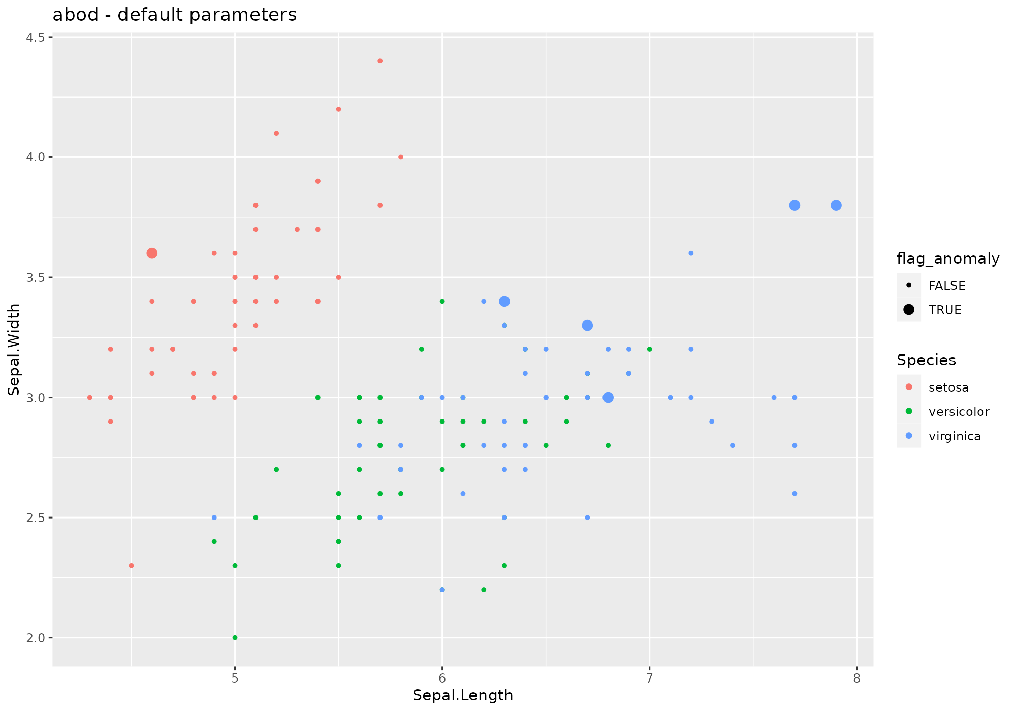

Default values for abod parameters:

k=10
… additional parameters to be passed to abod (method and n_sample_size - see ?abod.

Extra parameters used in stranger for this weird: none.

Default naming convention for generated metric based on k.

NOTE: this method is not recommended for volumetric data.

From abod help:

Details

Please note that ‘knn’ has to compute an euclidean distance matrix before computing abof.

Value

Returns angle-based outlier factor for each observation. A small abof respect the others would indicate presence of an outlier.

autoencode

## *** weird method autoencode
## autoencode based on function autoencode [autoencoder]
## Metric: Positive numeric value (probability) sorted in decreasing order.

iris %>% 
  lucky_odds(n.anom=6, analysis.drop="Species", weird="autoencode") %>%
  anoplot(title="autoencode - default parameters")

## Loading required package: autoencoder

## autoencoding...
## Optimizer counts:
## function gradient 
##      182       46 
## Optimizer: successful convergence.
## Optimizer: convergence = 0, message = 
## J.init = 41.81867, J.final = 0.3667237, mean(rho.hat.final) = 0.001268951

## Warning: Using size for a discrete variable is not advised.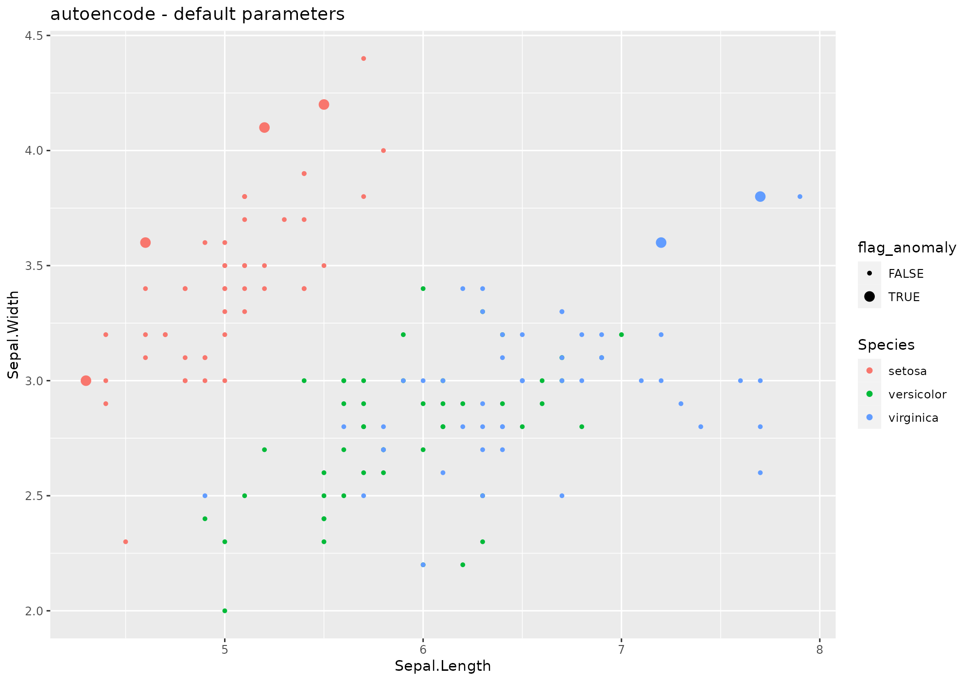

Changing some parameters:

iris %>%
  lucky_odds(n.anom=6, analysis.drop="Species", weird="autoencode",nl=4, N.hidden=c(10,8),beta=6) %>%
  anoplot(title="autoencode - change network layers strucure")

## autoencoding...
## Optimizer counts:
## function gradient 
##       27        3 
## Optimizer: successful convergence.
## Optimizer: convergence = 0, message = 
## J.init = 41.8159, J.final = 1.626769, mean(rho.hat.final) = 1.75171e-12

## Warning: Using size for a discrete variable is not advised.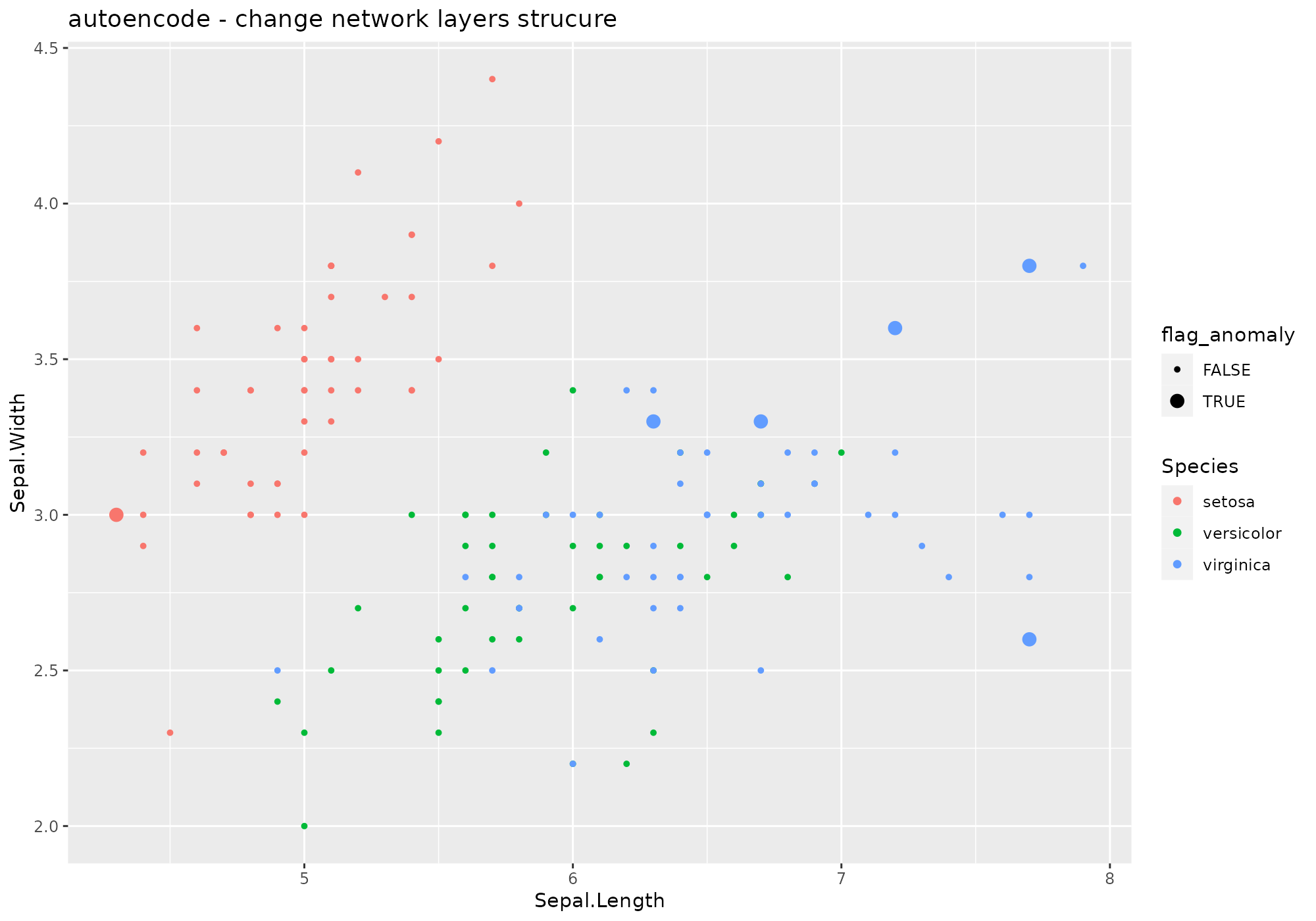

Default values for autoencode parameters:

nl=3
N.hidden=10
unit.type=“tanh”
lambda=0.0002
beta=6
rho=0.001
epsilon=0.0001
optim.method=“BFGS”
max.iterations=100
rescale.flag=TRUE
…: user may pass other parameters to autoencode (rescaling.offset).

Extra parameters used in stranger for this weird: none.

Default naming convention for generated metric based on nl and n.hidden.

From autoencode package: An autoencoder neural network is an unsupervised learning algorithm that applies backpropagation to adjust its weights, attempting to learn to make its target values (outputs) to be equal to its inputs. In other words, it is trying to learn an approximation to the identity function, so as its output is similar to its input, for all training examples. With the sparsity constraint enforced (requiring that the average, over training set, activation of hidden units be small), such autoencoder automatically learns useful features of the unlabeled training data, which can be used for, e.g., data compression (with losses), or as features in deep belief networks.

Usage here is to learn an autoencoder then apply it to same data and look at high residuals.

isofor

## *** weird method isolation Forest
## isofor based on function iForest [isofor]
## Metric: Positive numeric value (distance) sorted in decreasing order.

iris %>% 
  lucky_odds(n.anom=6, analysis.drop="Species", weird="isofor") %>%
  anoplot(title="isofor - default parameters")

## Loading required package: isofor

## Warning: Using size for a discrete variable is not advised.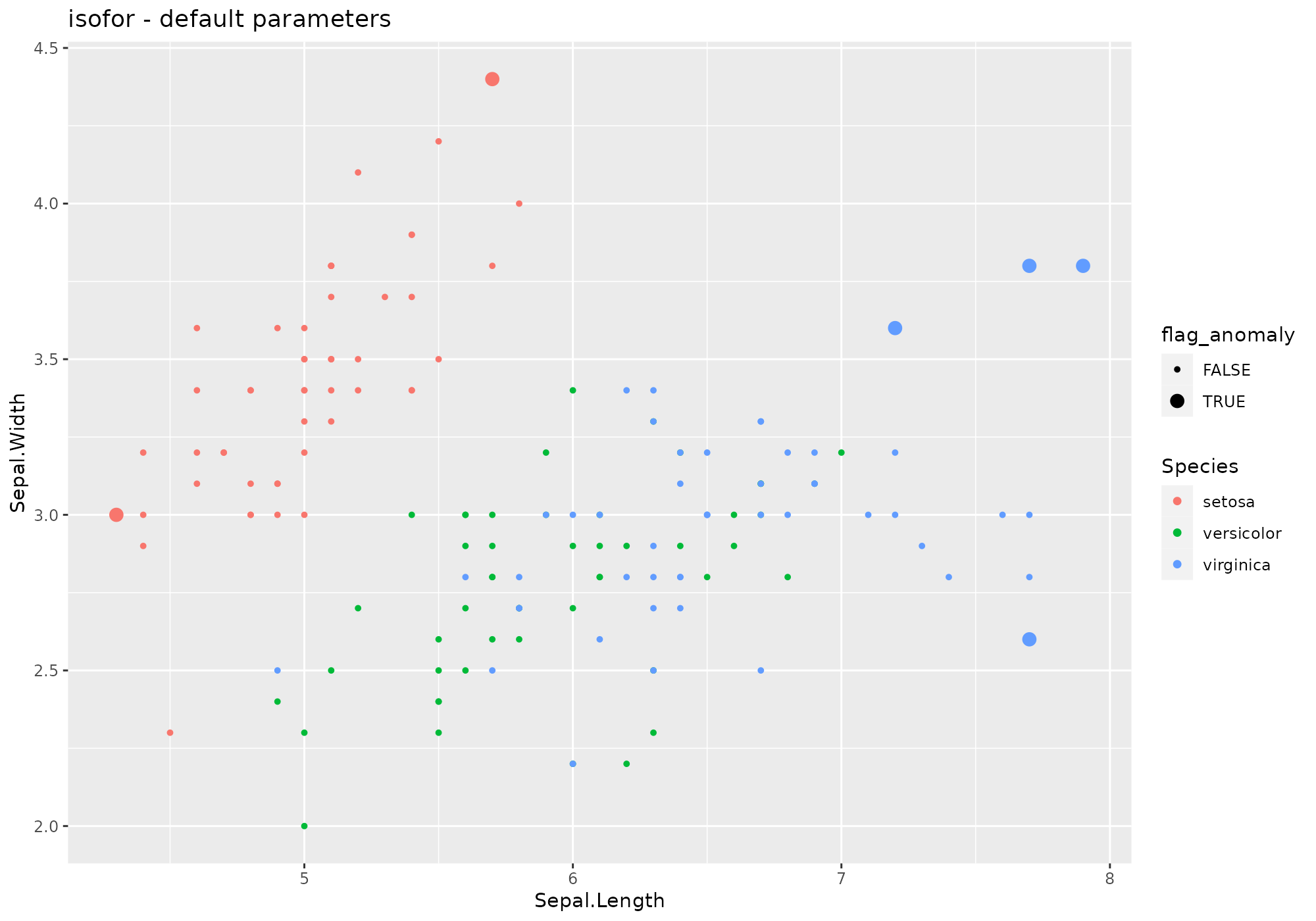

Default values for abod parameters – see ?iForest:

nt=100
phi=min(nrow(data)-1,256)
seed=1234
multicore=FALSE
replace_missing=TRUE
sentinel=-9999999999

Extra parameters used in stranger for this weird: none.

Default naming convention for generated metric based on nt and phi.

NOTE: this method is not recommended for volumetric data.

From iForest help:

An Isolation Forest is an unsupervised anomaly detection algorithm. The requested number of trees, nt, are built completely at random on a subsample of size phi. At each node a random variable is selected. A random split is chosen from the range of that variable. A random sample of factor levels are chosen in the case the variable is a factor.

Records from X are then filtered based on the split criterion and the tree building begins again on the left and right subsets of the data. Tree building terminates when the maximum depth of the tree is reached or there are 1 or fewer observations in the filtered subset.

kmeans

## *** weird method kmeans ()
## kmeans based on function kmeans [stats]
## Metric: Positive numeric value (distance) sorted in decreasing order.

iris %>% 
  lucky_odds(n.anom=6, analysis.drop="Species", weird="kmeans") %>%
  anoplot(title="kmeans - default parameters")

## Warning: Using size for a discrete variable is not advised.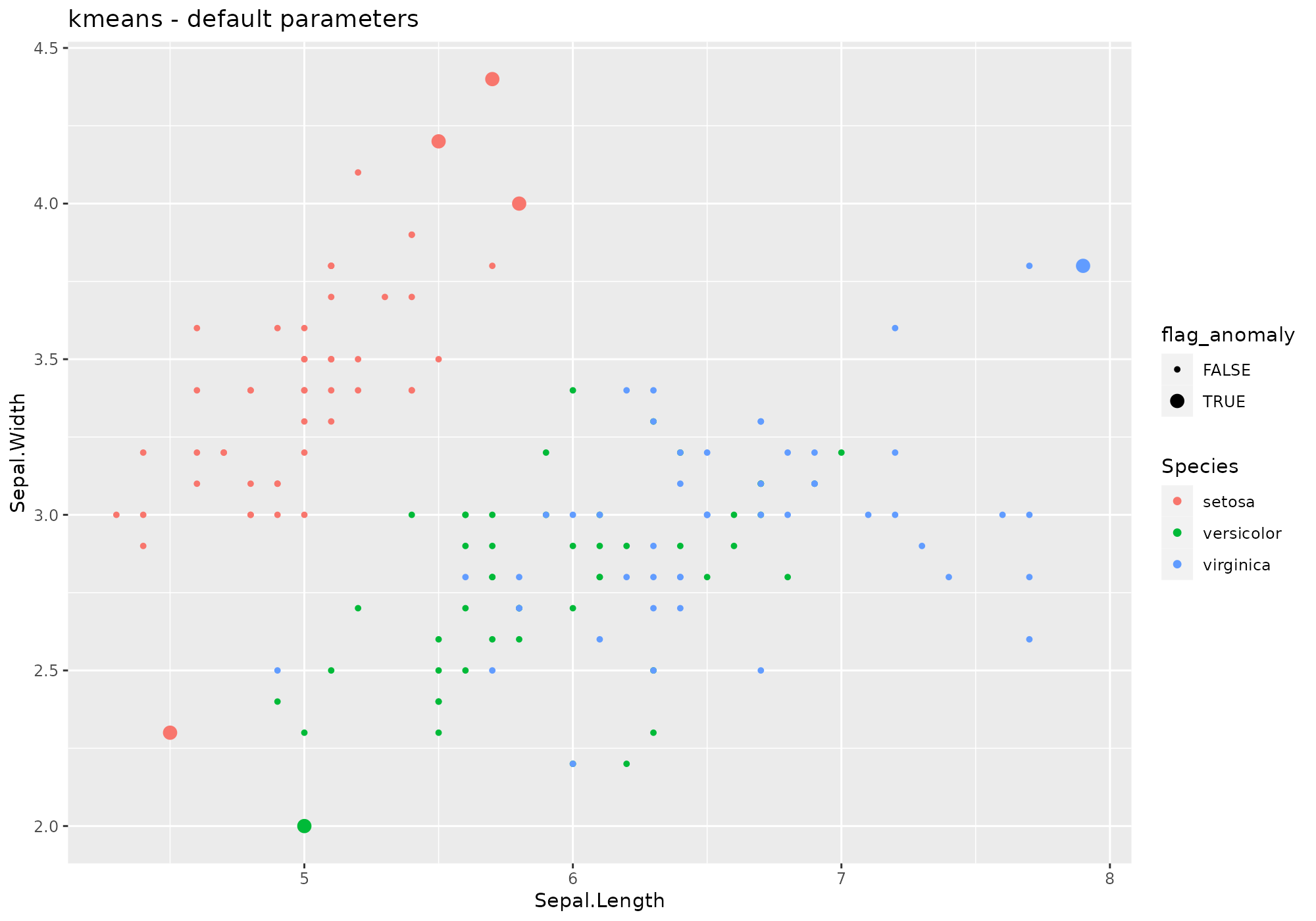

Default values for kmeans parameters – see ?kmeans:

type=“means”
centers=4
algorithm=“Hartigan-Wong”
iter.max=10
nstart= centers parameter (4)

Extra parameters used in stranger for this weird: none.

Default naming convention for generated metric based on type and centers.

iris %>% 
  lucky_odds(n.anom=6, analysis.drop="Species",weird="kmeans",type="euclidian",centers=8) %>% 
  anoplot(title="kmeans - euclidean - nclusters (centers)=8")

## Warning: Using size for a discrete variable is not advised.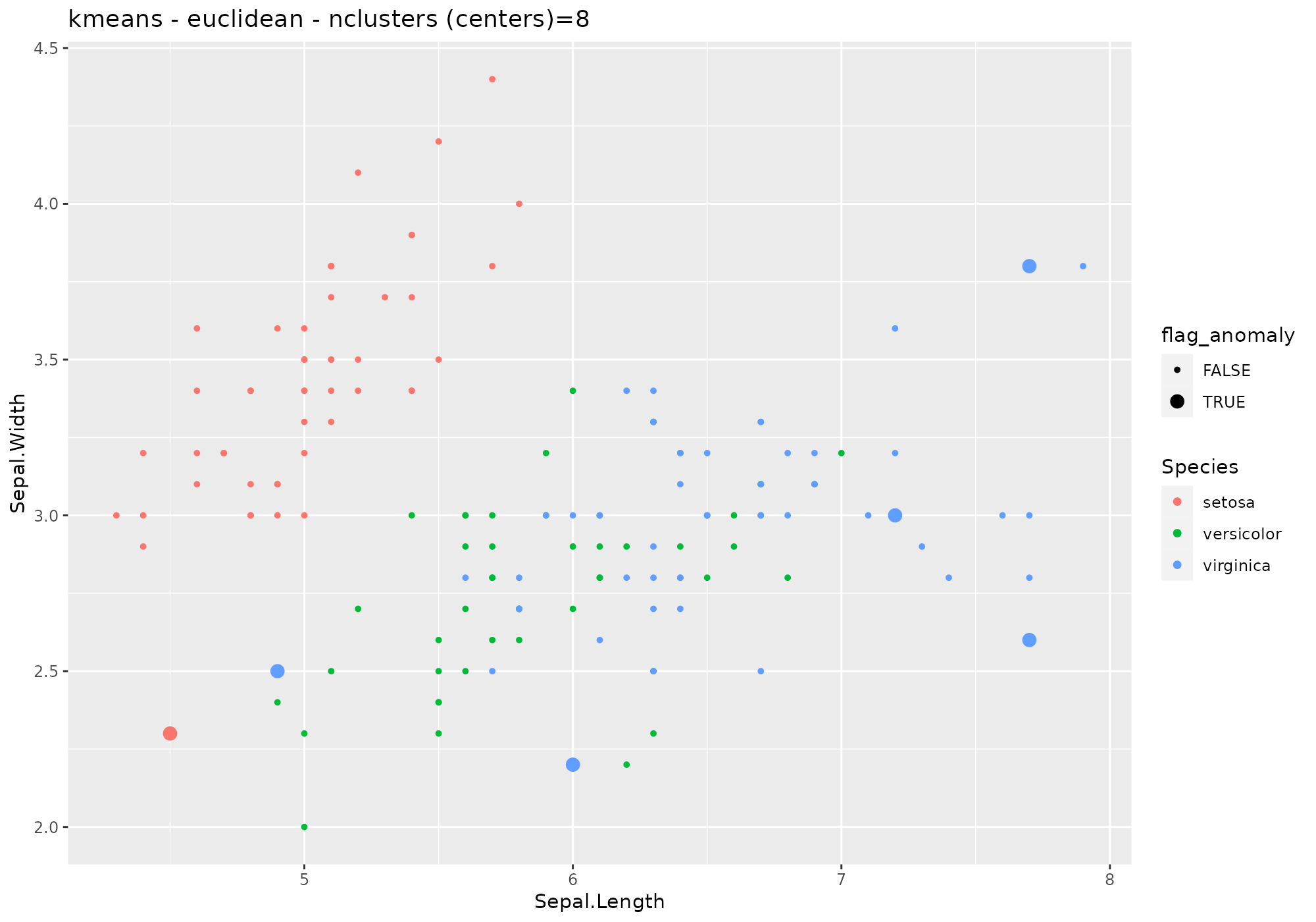

iris %>% 
  lucky_odds(n.anom=6, analysis.drop="Species",weird="knn",simplify="median") %>% 
  anoplot(title="knn - k=default (10), simplify=median")

## Loading required package: FNN

## Warning: Using size for a discrete variable is not advised.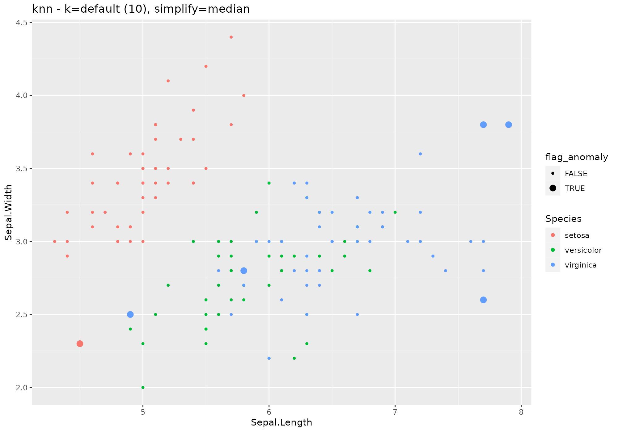

knn

## *** weird method k-Nearest Neighbour
## knn based on function knn.dist [FNN]
## Metric: Positive numeric value (distance) sorted in decreasing order.

iris %>% 
  lucky_odds(n.anom=6, analysis.drop="Species", weird="knn") %>%
  anoplot(title="knn - default parameters")

## Warning: Using size for a discrete variable is not advised.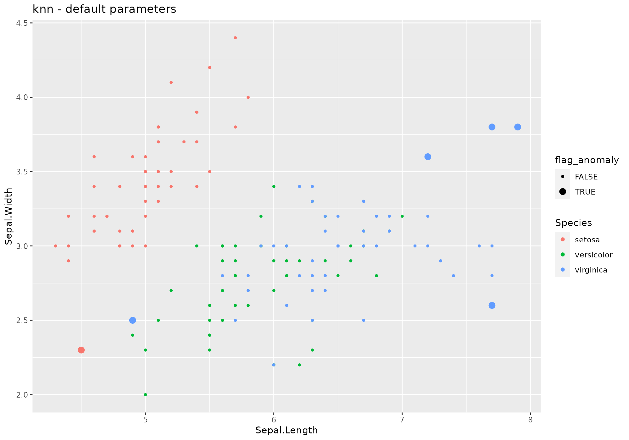

Default values for knn parameters – see ?knn:

k=10
… other parameters to be passed to knn (prob, algorihtm)

Extra parameters used in stranger for this weird:

simplify=“mean”: name of a function to be used to aggregate neirest neighbours distances. User may use other existing base funcions (for instance median) but can also use his own function – name to be supplied as string.

Default naming convention for generated metric based on k and simplify.

iris %>% 
  lucky_odds(n.anom=6, analysis.drop="Species",weird="knn",k=8) %>% 
  anoplot(title="knn - k=8")

## Warning: Using size for a discrete variable is not advised.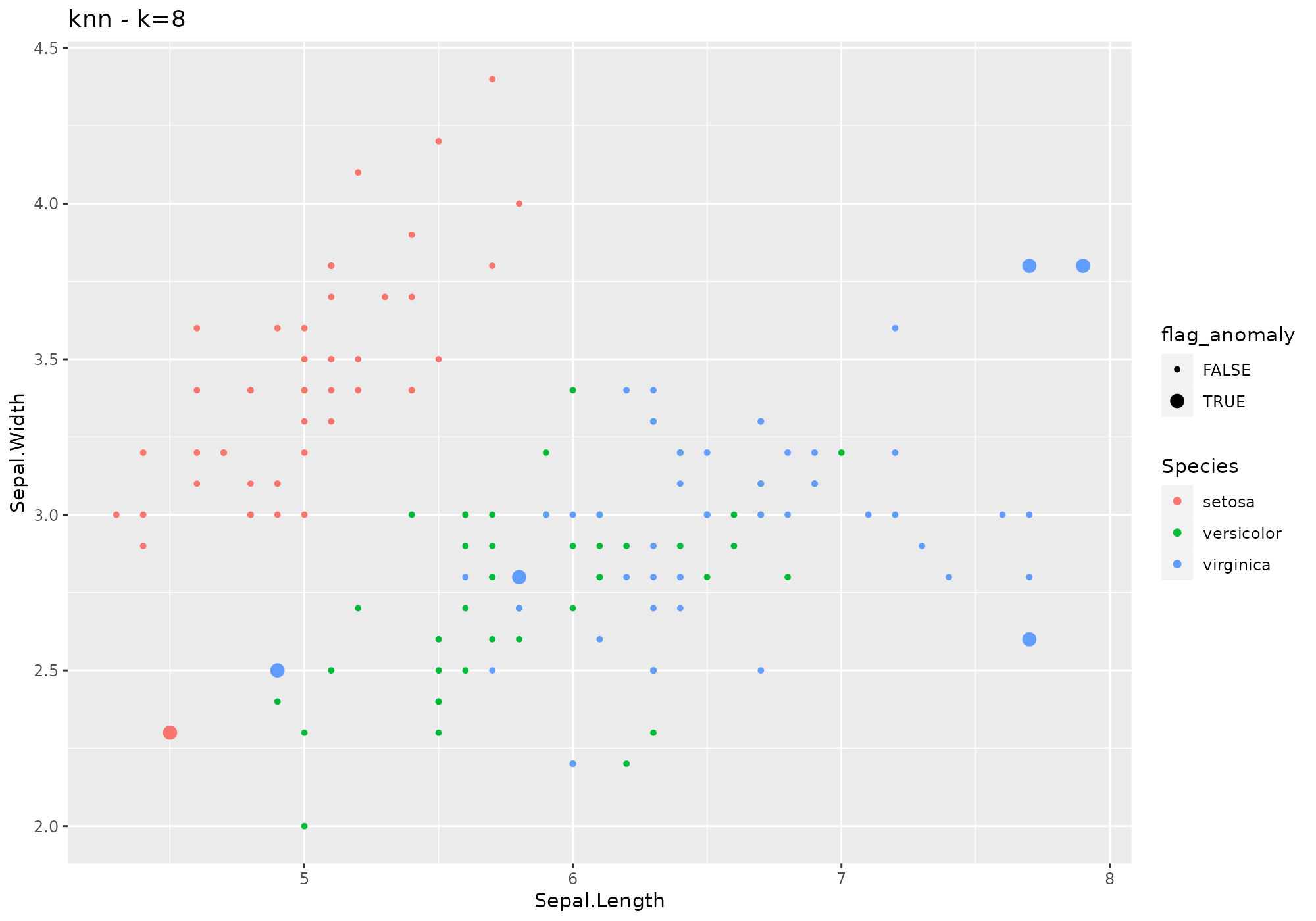

iris %>% 
  lucky_odds(n.anom=6, analysis.drop="Species",weird="knn",simplify="median") %>% 
  anoplot(title="knn - k=default (10), simplify=median")

## Warning: Using size for a discrete variable is not advised.

lof

## *** weird method Local Outlier Factor
## lof based on function lof [dbscan]
## Metric: Positive numeric value (local outlier factors) sorted in decreasing order.

iris %>% 
  lucky_odds(n.anom=6, analysis.drop="Species", weird="lof") %>%
  anoplot(title="lof - default parameters")

## Loading required package: dbscan

## Warning: Using size for a discrete variable is not advised.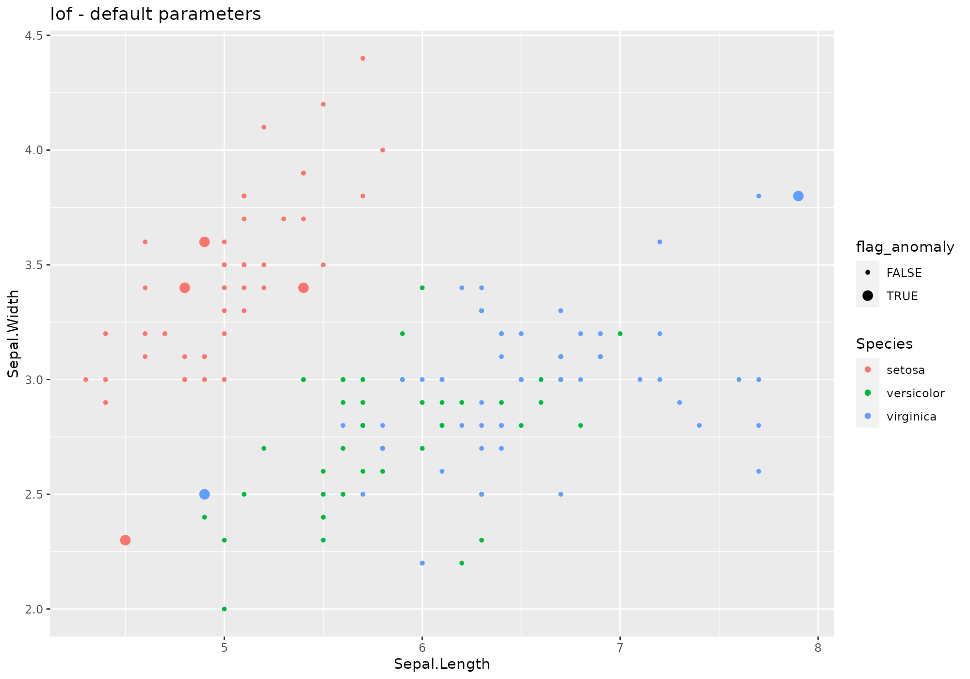

Default values for lof parameters – see ?lof:

minPts=5
… other parameters to be passed to kNN from dbscan package (search, bucketSize…).

Extra parameters used in stranger for this weird: none.

Default naming convention for generated metric based on minPts.

iris %>% 
  lucky_odds(n.anom=6, analysis.drop="Species",weird="lof",minPts=5, search="linear") %>% 
  anoplot(title="lof - minPts=8 - linear kNN")

## Warning: Using size for a discrete variable is not advised.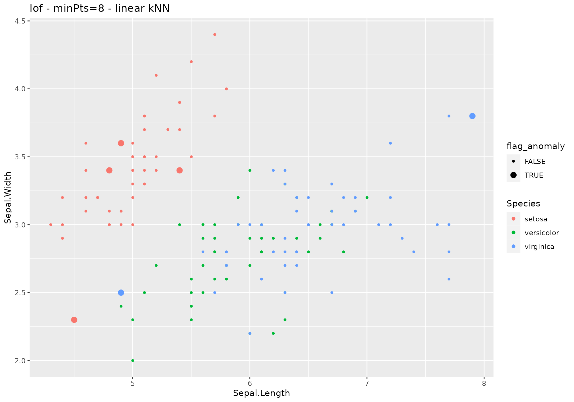

From lof help:

LOF compares the local density of an point to the local densities of its neighbors. Points that have a substantially lower density than their neighbors are considered outliers. A LOF score of approximately 1 indicates that density around the point is comparable to its neighbors. Scores significantly larger than 1 indicate outliers.

mahalanobis

## *** weird method Mahalanobis distance
## mahalanobis based on function mahalanobis [stats]
## Metric: Positive numeric value (distance) sorted in decreasing order.

iris %>% 
  lucky_odds(n.anom=6, analysis.drop="Species", weird="mahalanobis") %>%
  anoplot(title="mahalanobis - default parameters")

## Warning: Using size for a discrete variable is not advised.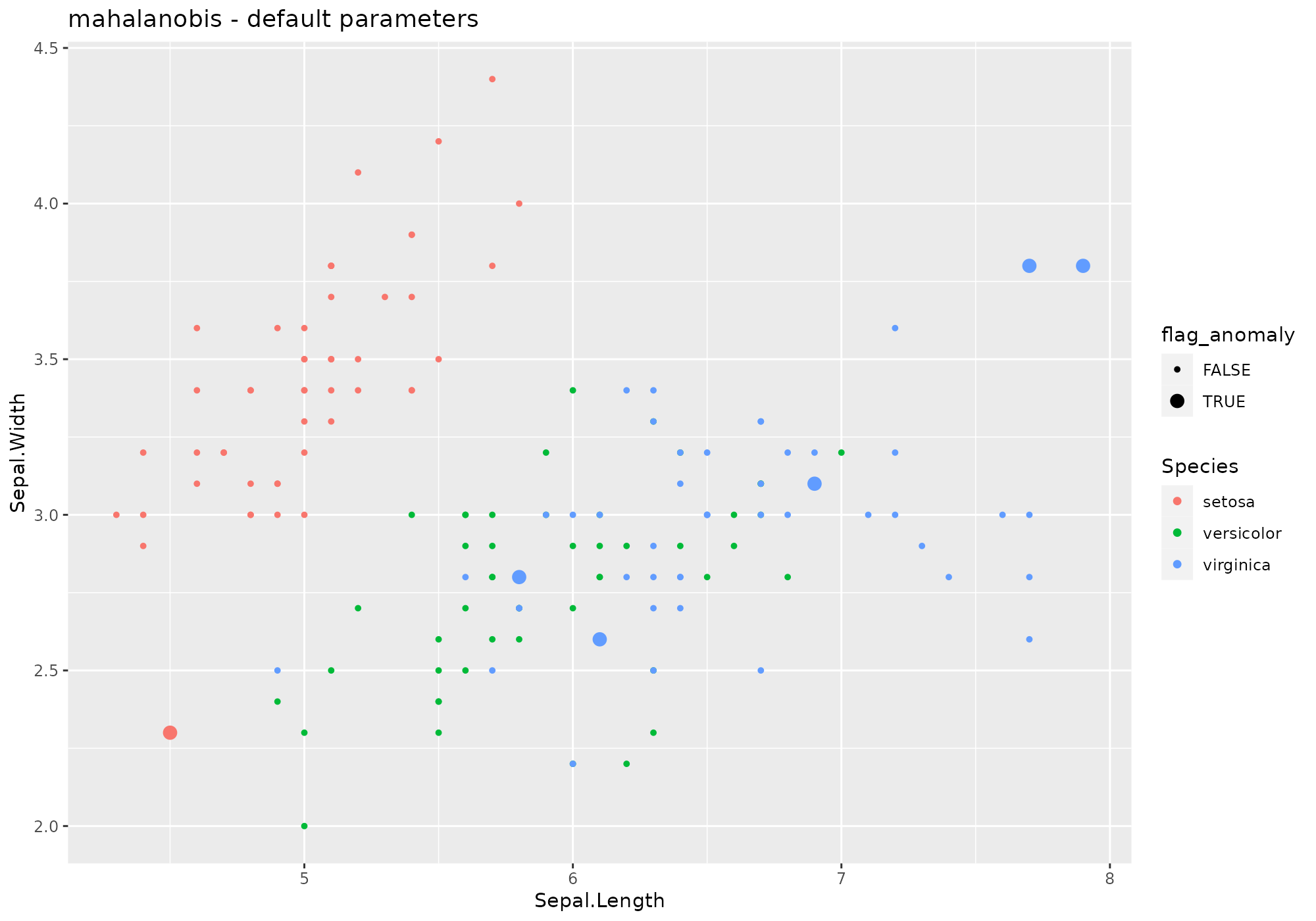

No parameter available.

Default naming convention: mahalanobis.

pcout

## *** weird method Semi-robust principal components > distances
## pcout based on function pcout [mvoutlier]
## Metric: Positive numeric value (distance) sorted in decreasing order.

iris %>% 
  lucky_odds(n.anom=6, analysis.drop="Species", weird="pcout") %>%
  anoplot(title="pcout - default parameters")

## Loading required package: mvoutlier

## Loading required package: sgeostat

## Warning: Using size for a discrete variable is not advised.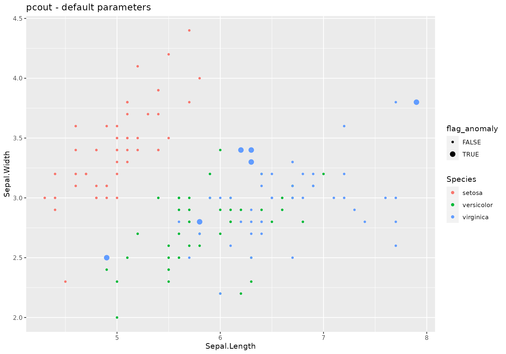

Default values for pcout parameters – see ?pcout:

explvar=0.99
crit.M1=1/3
crit.M2=1/4
crit.c2=0.99
crit.cs=0.25
outbound=0.25
… not used here.

Extra parameters used in stranger for this weird: none.

Default naming convention for generated metric based on explvar.

iris %>% 
  lucky_odds(n.anom=6, analysis.drop="Species",weird="pcout", explvar=0.8, crit.Ml=1, crit.cl=3) %>% 
  anoplot(title="pcout - custom values")

## Warning: Using size for a discrete variable is not advised.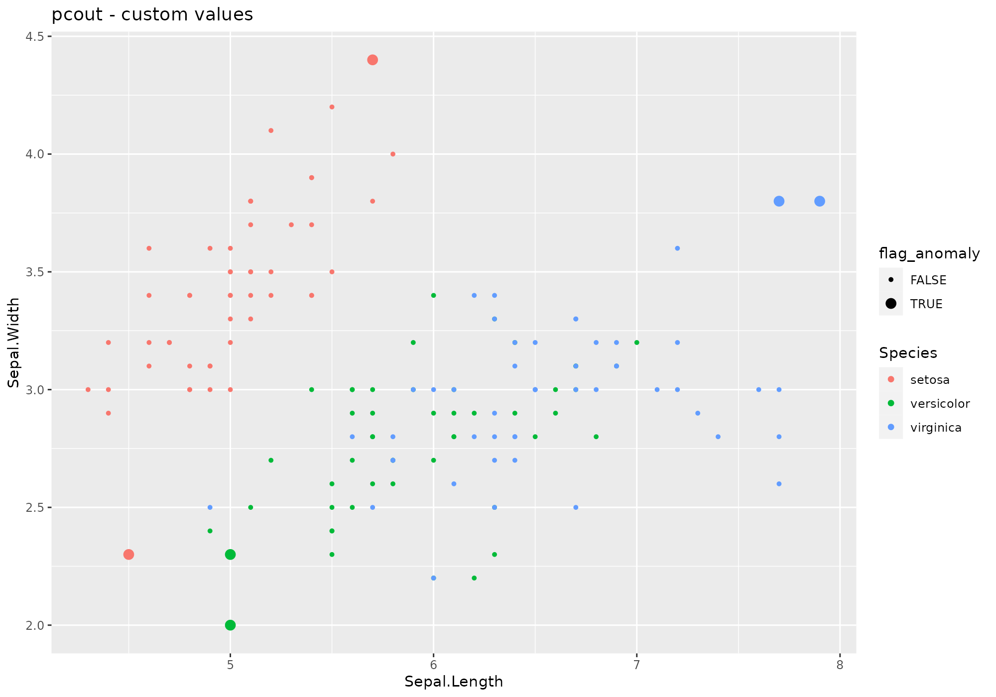

From pcout help:

Based on the robustly sphered data, semi-robust principal components are computed which are needed for determining distances for each observation. Separate weights for location and scatter outliers are computed based on these distances. The combined weights are used for outlier identification.

randomforest

## *** weird method randomforest outlier metric
## randomforest based on function randomForest [randomForest]
## Metric: Positive numeric value (distance) sorted in decreasing order.

iris %>% 
  lucky_odds(n.anom=6, analysis.drop="Species", weird="randomforest") %>%
  anoplot(title="randomforest - default parameters")

## Loading required package: randomForest

## randomForest 4.7-1.1

## Type rfNews() to see new features/changes/bug fixes.

## 
## Attaching package: 'randomForest'

## The following object is masked from 'package:ggplot2':
## 
##     margin

## The following object is masked from 'package:dplyr':
## 
##     combine

## Warning: Using size for a discrete variable is not advised.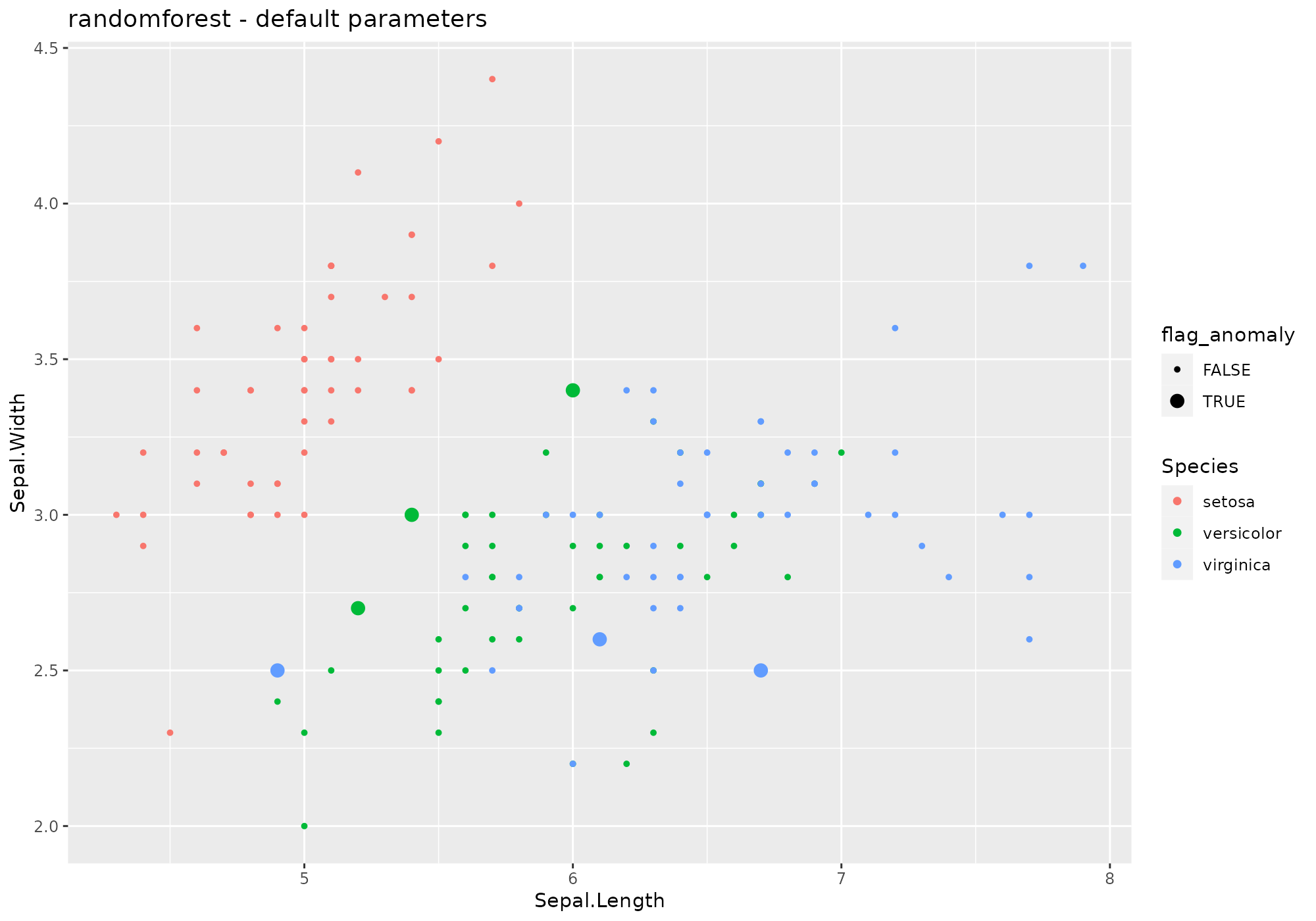

Default values for randomforest parameters – see ?randomforest:

ntree=500
mtry=sqrt(ncol(data))
replace=TRUE
… other parameters to be used in randomForest

Extra parameters used in stranger for this weird: none.

Default naming convention for generated metric based on ntree and mtry.

iris %>% 
  lucky_odds(n.anom=6, analysis.drop="Species",weird="randomforest", explvar=0.8, ntree=10,mtry=2) %>% 
  anoplot(title="randomforest - custom values")

## Warning: Using size for a discrete variable is not advised.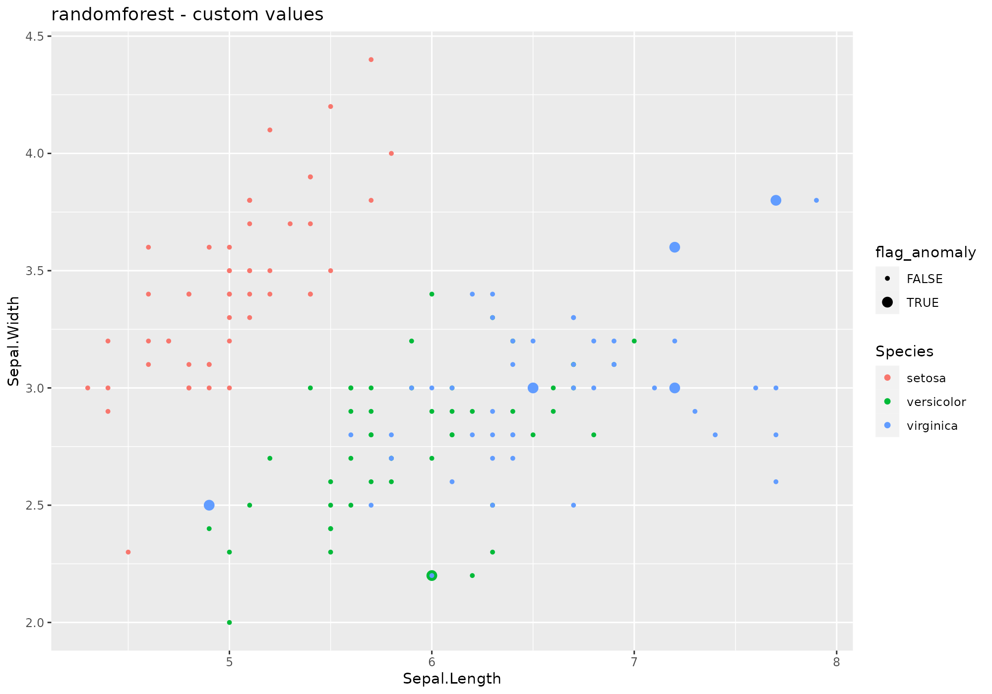

To go further

Logical next step is to look at how to work with weirds methods: manipulate, work with metrics (aggregation and stacking), derive anomalies. For this, read vignette Working with weirds

WeLoveDataScience

2022-10-08

abod

autoencode

isofor

kmeans

knn

lof

mahalanobis

pcout

randomforest

To go further