working with weirds
WeLoveDataScience
2022-10-08
working_with_weirds.RmdAnomalies manual selection
For some metrics, litterature recommends some cutpoints (2 for
lof for instance).
There is a way to derive anomalies from this given cutpoint by filtering a stranger or a singularize object and convert to anomalies the set of retained records.
Filtering can be done either with usual [ or
dplyr select.
Assumed dbscan package is installed, one can for
instance use lof weird, use 2 as cutpoint and derive an
anomaly object with as.anomalies.
## Loading required package: dbscan
anom <- filter(s,lof_minPts_5>2) %>% as.anomalies()Anomaly objects are simple vectors with attributes; once can then access the first anomaly and display it with:
plot(s,type="neighbours", score="lof_minPts_5",anomaly_id=anom[1])## Your data has been converted to a dataframe to be compatible with ggplot function.## Loading required package: FNN## `geom_smooth()` using formula 'y ~ x'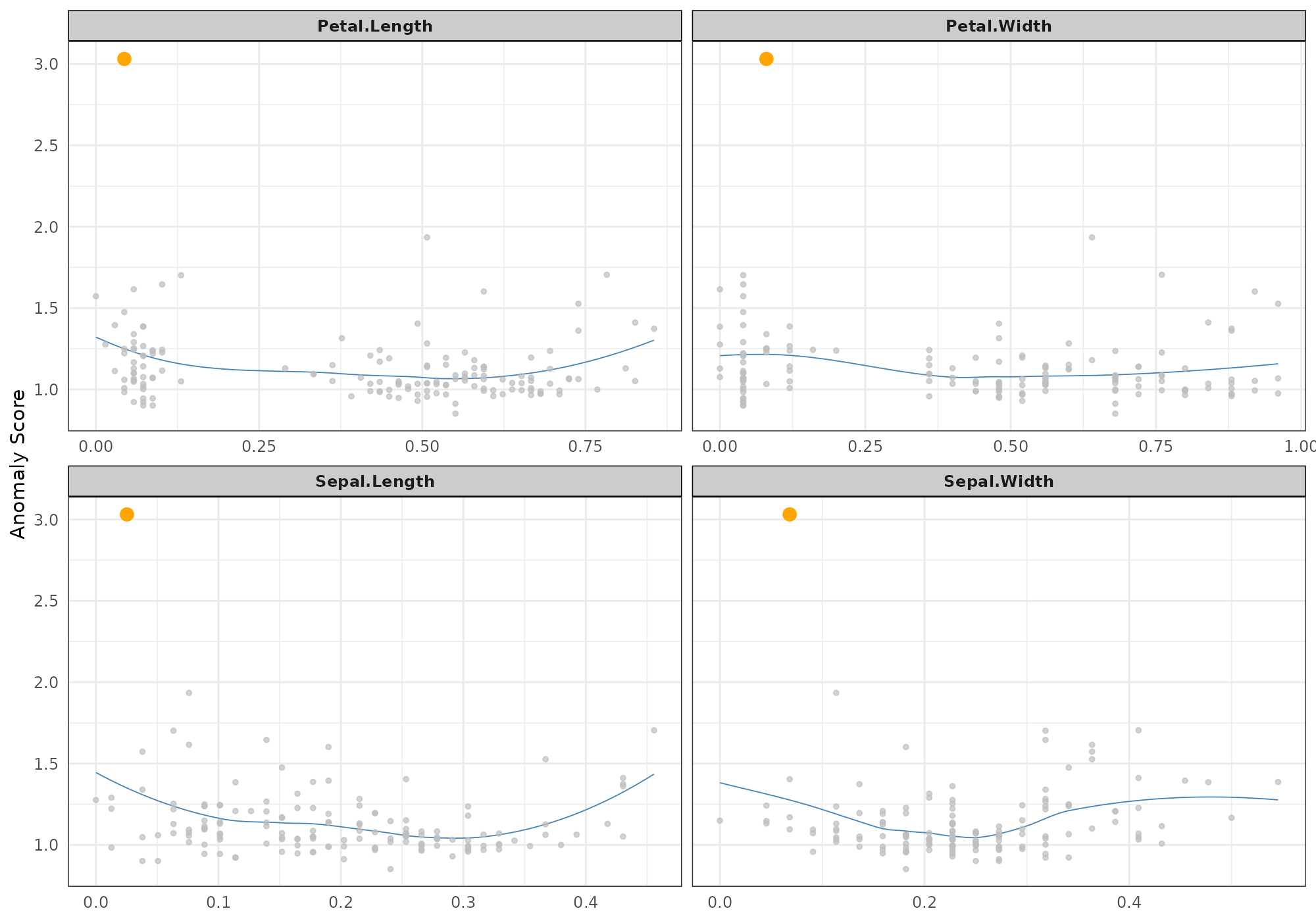
Using a tuneGrid
stranger package is a wrapper around several methods.
Problem thus arrives on the choice of the method… We will see
later in this vignette how to work with several metrics and in
particular the stacking.
But world is really complex and even for one chosen method, leyt say
knn weird, user has to pick some parameters…
Here comes the parameter tuneGrid (name borrowed from
caret) that allow to use one weird with different
sets of parameters in the same call.
Let’s prepare a matrix of parameters:
tg <- expand.grid(k=c(5,10,20),simplify=c("mean","median"),stringsAsFactors=FALSE)
tg
## k simplify
## 1 5 mean
## 2 10 mean
## 3 20 mean
## 4 5 median
## 5 10 median
## 6 20 medianWe thus have 6 possible combinations
##      .id knn_k_5_mean knn_k_10_mean knn_k_20_mean knn_k_5_median
##   1:   1   0.02560115    0.03647553    0.05368046     0.02601460
##   2:   2   0.03628835    0.04448610    0.06322990     0.03894765
##   3:   3   0.03605785    0.04354593    0.05611057     0.03894765
##   4:   4   0.03256554    0.04072704    0.05649871     0.02977918
##   5:   5   0.03984542    0.04519420    0.05902922     0.04195510
##  ---
## 146: 146   0.07056222    0.08621572    0.11121305     0.07400789
## 147: 147   0.07533194    0.10077827    0.12428750     0.07925859
## 148: 148   0.07167463    0.08622770    0.10228438     0.07429926
## 149: 149   0.08643839    0.10152256    0.12754738     0.10533133
## 150: 150   0.06003996    0.07692173    0.10060785     0.06290052
##      knn_k_10_median knn_k_20_median
##   1:      0.03488959      0.05278479
##   2:      0.04426191      0.05939418
##   3:      0.04408645      0.05960504
##   4:      0.04182115      0.05447469
##   5:      0.04771224      0.05636842
##  ---
## 146:      0.09178279      0.11484551
## 147:      0.10273185      0.13174353
## 148:      0.08791375      0.10983492
## 149:      0.11319301      0.12104827
## 150:      0.08442104      0.10450279
NOTES
-
strangernaming conventions do not necessary involve all parameters, we though ensure unique names and store parameters values as attributes (metadata) for every metric. - Currently, only parameters exposed in weird method are
allowed in tuning grid. User can still invoke methods several times with
different values for other parameters and merge results as seen in next
section or use
stranger.
tg = data.frame(k=c(5,5:8))
(anoms <-  iris %>% select(-Species) %>%
  crazyfy() %>% strange(weird="knn",tuneGrid=tg,algorithm=c("cover_tree")))
## .id knn_k_5_mean knn_k_5_mean.1 knn_k_6_mean knn_k_7_mean knn_k_8_mean
## 1: 1 0.02560115 0.02560115 0.02800096 0.03034193 0.03244721
## 2: 2 0.03628835 0.03628835 0.03800174 0.03946357 0.04128187
## 3: 3 0.03605785 0.03605785 0.03749732 0.03879323 0.04027742
## 4: 4 0.03256555 0.03256555 0.03458706 0.03603100 0.03734822
## 5: 5 0.03984543 0.03984543 0.04115709 0.04216815 0.04306710
## ---
## 146: 146 0.07056224 0.07056224 0.07412305 0.07668065 0.07947144
## 147: 147 0.07533194 0.07533194 0.08271409 0.08860528 0.09333819
## 148: 148 0.07167465 0.07167465 0.07490411 0.07773136 0.08103779
## 149: 149 0.08643838 0.08643838 0.09089748 0.09425377 0.09678463
## 150: 150 0.06003996 0.06003996 0.06483095 0.06838887 0.07124970
(meta <- get_info(anoms))## weird_method name package package.source foo
## knn_k_5_mean "k-Nearest Neighbour" "knn" "FNN" "CRAN" "knn.dist"
## knn_k_5_mean.1 "k-Nearest Neighbour" "knn" "FNN" "CRAN" "knn.dist"
## knn_k_6_mean "k-Nearest Neighbour" "knn" "FNN" "CRAN" "knn.dist"
## knn_k_7_mean "k-Nearest Neighbour" "knn" "FNN" "CRAN" "knn.dist"
## knn_k_8_mean "k-Nearest Neighbour" "knn" "FNN" "CRAN" "knn.dist"
## type sort detail parameters
## knn_k_5_mean "distance" -1 "Positive numeric value (distance)" list,3
## knn_k_5_mean.1 "distance" -1 "Positive numeric value (distance)" list,3
## knn_k_6_mean "distance" -1 "Positive numeric value (distance)" list,3
## knn_k_7_mean "distance" -1 "Positive numeric value (distance)" list,3
## knn_k_8_mean "distance" -1 "Positive numeric value (distance)" list,3
## normalizationFunction colname
## knn_k_5_mean ? "knn_k_5_mean"
## knn_k_5_mean.1 ? "knn_k_5_mean"
## knn_k_6_mean ? "knn_k_6_mean"
## knn_k_7_mean ? "knn_k_7_mean"
## knn_k_8_mean ? "knn_k_8_mean"
meta[,"parameters"]## $knn_k_5_mean
## $knn_k_5_mean$k
## [1] 5
##
## $knn_k_5_mean$algorithm
## [1] "cover_tree"
##
## $knn_k_5_mean$simplify
## [1] "mean"
##
##
## $knn_k_5_mean.1
## $knn_k_5_mean.1$k
## [1] 5
##
## $knn_k_5_mean.1$algorithm
## [1] "cover_tree"
##
## $knn_k_5_mean.1$simplify
## [1] "mean"
##
##
## $knn_k_6_mean
## $knn_k_6_mean$k
## [1] 6
##
## $knn_k_6_mean$algorithm
## [1] "cover_tree"
##
## $knn_k_6_mean$simplify
## [1] "mean"
##
##
## $knn_k_7_mean
## $knn_k_7_mean$k
## [1] 7
##
## $knn_k_7_mean$algorithm
## [1] "cover_tree"
##
## $knn_k_7_mean$simplify
## [1] "mean"
##
##
## $knn_k_8_mean
## $knn_k_8_mean$k
## [1] 8
##
## $knn_k_8_mean$algorithm
## [1] "cover_tree"
##
## $knn_k_8_mean$simplify
## [1] "mean"Merging stranger objects
So you have decided to go for and try two different methods. Let say knn and autoencode.
First, we can create two object containg assciatdd metrics.
data <- iris %>% select(-Species) %>% crazyfy()
m1 <- strange(data, weird="knn")
m2 <- strange(data, weird="autoencode")
## Loading required package: autoencoder## autoencoding...
## Optimizer counts:
## function gradient
## 147 58
## Optimizer: successful convergence.
## Optimizer: convergence = 0, message =
## J.init = 41.81819, J.final = 0.3576837, mean(rho.hat.final) = 0.001328208For convenience and further exploitation, a merge method
is at your disposal to gather the two corresponding metrics in a single
object:
(metrics <- merge(m1,m2))## .id knn_k_10_mean autoencode_nl_3_Nhidden_10
## 1: 1 0.03647553 0.06897433
## 2: 2 0.04448610 0.06770391
## 3: 3 0.04354593 0.07207966
## 4: 4 0.04072704 0.06799357
## 5: 5 0.04519420 0.07090437
## ---
## 146: 146 0.08621572 0.05330294
## 147: 147 0.10077827 0.03176485
## 148: 148 0.08622770 0.03619777
## 149: 149 0.10152256 0.05480954
## 150: 150 0.07692173 0.02408043Invoke several weirds at once (stranger)
You are not sure yet about the metric you want to use. Or you would
like to test many, with plenty of different values for the parameters?
stranger is for you. This function is similar to
caretList in caretEnsemble package.
With its first parameter weirdList you can supply many methods that will be invoked with their default parameter.
If you want to use your own values or use a tuneGrid for a given
method, you will have to create weird objects using
weird function and pass a list of such weirds
object to the parameter tuneList.
Following call will for instance: * fit a knn weird with default values (taken from weirdList) * fit a autoencode weird with default values * also fit a knn but with k set to 20 (not recommended for iris data having 50 observations)
## autoencoding...
## Optimizer counts:
## function gradient
##      102       39
## Optimizer: successful convergence.
## Optimizer: convergence = 0, message =
## J.init = 41.81935, J.final = 0.3687884, mean(rho.hat.final) = 0.001198874